Linear function
In this article we study linear functions. We analyze their definition, characteristics, elements, special cases and applications. In addition, we look at several examples and graphs.
Table of Contents
Definition
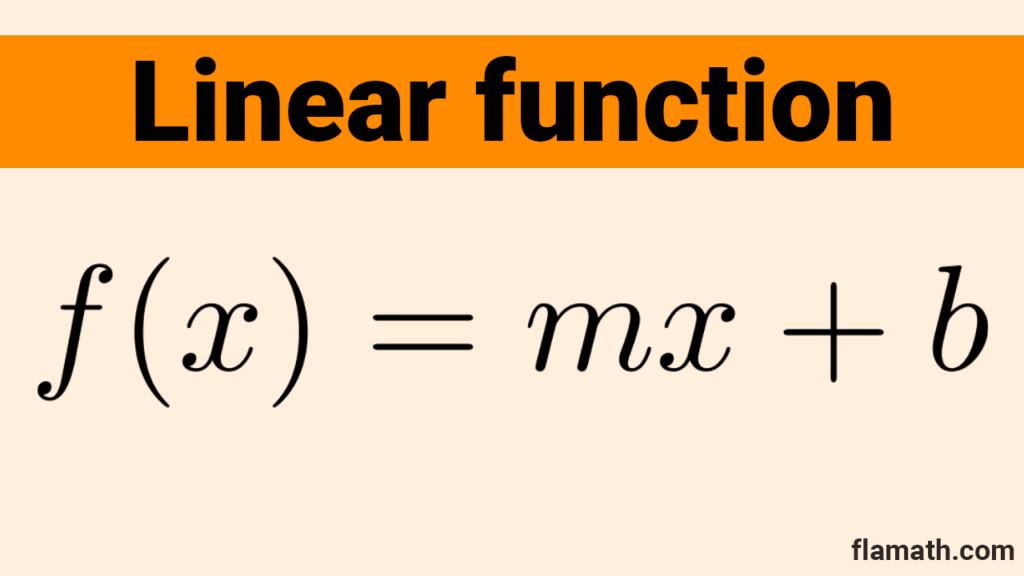
A linear function is an algebraic function of the form *f(x)=mx+b,* where m and b are any real numbers.
In other words, a linear function is a polynomial function of degree 1 (when m is different from zero) or degree 0 (when m equals zero). The term *mx* is called the linear term, where m is the coefficient of the term; the number b is called the constant term.
Some examples of linear functions are:
*y=2x+1*
*f(x)=-6*
*g(x)=-x*
*h(x)=-3x-6*
*v=3u+1*
Some literature refers to an affine function as a function of the form *f(x)=mx+b,* reserving the name "linear function" for the case where *b=0,* that is, *f(x)=mx* (this is also known as a function of direct proportionality). In this article, we will treat linear and affine functions as the same thing.
Characteristics and elements
A linear function is composed of several elements that describe its behavior and give it its special characteristics. These elements are:
- Variables.
- Domain.
- Range.
- Graph.
- Slope.
- Y-intercept.
- Root.
Variables
Independent variable: it is the variable used as input in the function. It represents the values that can vary within the function. Generally represented by the letter *x.*
Dependent variable: it is the output value resulting from applying the function to the independent variable. The dependent variable changes according to the values of the independent variable according to the defining rule. Generally represented by the letter *y* or *f(x).*
Domain and Range
The domain of a function is the set of all possible values that the independent variable can take. The range of a function is the set of all values that result from applying the function to each number in the domain.
The domain of a linear function is the set of real numbers, as it is a polynomial function and there are no restrictions for input values.
The range of a linear function is the set of real numbers (when m is different from zero) or the set whose only element is b: *\{b\}* (when m equals zero), the latter is because the function takes only one value for any element in the domain.
Graph
The graphical representation of a linear function is a straight line in a Cartesian coordinate system. This is why it is called "linear."
If we know the equation of a linear function, to graph it, it is enough to determine two of its points and draw the line that passes through them. In order to avoid errors, it is recommended to find several points before drawing the line. This way, any calculation error will be evident as the points will not be aligned.
Example: *f(x)=2x-3*
We find some points of the graph through a table of values:
| x | y=f(x) | (x, y) |
| -2 | 2(-2)-3= -7 | (-2, -7) |
| -1 | 2(-1)-3= -5 | (-1, -5) |
| 0 | 2(0)-3= -3 | (0, -3) |
| 1 | 2(1)-3= -1 | (1, -1) |
| 2 | 2(2)-3= 1 | (2, 1) |
In the last column, we see the points that we need to plot on a Cartesian plane:
Having confirmed that the points are aligned, we proceed to draw the line that passes through them and write the formula of the function we are representing. With that, our work is complete.
Slope
The slope of a linear function is the coefficient of the linear term, that is, the number *m.* This value indicates the inclination of the line representing the function in a Cartesian coordinate system.
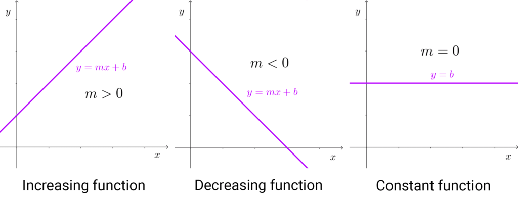
The slope also determines whether the linear function is increasing or decreasing: if it is positive, then the function is increasing; if it is negative, the function is decreasing. When the slope is zero, the function is neither increasing nor decreasing but constant.
In the following graph, we see how the slope affects the graph:
When we have the equation of a linear function, finding the slope involves determining the value that multiplies x (the independent variable). If x does not appear in the equation, it means the slope is zero.
Examples:
- The function *y=2x+1* has a slope of 2; as it is a positive number, the function is increasing.
- *f(x)=-6* has a slope of 0, as the independent variable is not visible in the equation. Therefore, the function is constant.
- *g(x)=-x-1* has a slope of -1; being a negative number, the linear function is decreasing.
We can also find the slope of a linear function from its graph. For this, we use the following property.
If we take two points on a line, *(x_1,y_1)* and *(x_2,y_2),* calculate the difference between the y values: *Δy=y_2-y_1* and the difference between the x values: *Δx=x_2-x_1,* and then perform the quotient *\dfrac{Δy}{Δx},* we will find that this number coincides with the slope of the line. That is, the slope of a linear function is the ratio between the variation in *y* and the variation in *x:*
*m=\dfrac{Δy}{Δx}=\dfrac{y_2-y_1}{x_2-x_1}*
Example:
We want to determine the slope of a linear function that passes through the points *(-2,-7)* and *(-1,-5).* To do this, we calculate the variations:
*Δy=y_2-y_1=-5-(-7)=2*
*Δx=x_2-x_1=-1-(-2)=1*
With these numbers, we find the quotient: *\dfrac{Δy}{Δx}=\dfrac{2}{1}=2*
Therefore, the slope we were looking for is *m=2.*
Y-Intercept
The y-intercept of a linear function is the value of its constant term. Graphically, it represents the point where the graph intersects the y-axis (when x equals zero).
To find the y-intercept, simply identify the term in the equation that does not contain x. A linear function always has a y-intercept. If it is not visible in the equation, it means it equals zero.
Examples
- The function *y=2x+1* has a y-intercept of *1.*
- *f(x)=-6* has a y-intercept of *-6.*
- *g(x)=-x-1* has a y-intercept of *-1.*
- *h(x)=2x* has a y-intercept equal to *0.*
To graphically find the y-intercept, it is necessary to determine the point where the line intersects the vertical axis. Note that in a function *f(x)=mx+b* when *x=0,* it follows that
*f(0)=m(0)+b→f(0)=b.*
Therefore, the graph of a linear function intersects the y-axis at the point *(0,b),* where b is the y-intercept.
For example, the graph of the following function intersects the vertical axis at *1,* which is its y-intercept. This data matches what we would obtain by examining the equation.
Zero
The zero or root of a linear function is the x-coordinate of the point where the graph intersects the x-axis.
To calculate the zero of the function, set the equation equal to *0* and solve for *x:*
*mx+b=0→x=-\dfrac{b}{m}*
Therefore, the graph intersects the x-axis at the point *(-b/m,0),* and the root of the function is the value *x=-\dfrac{b}{m}.* It is not necessary to memorize this formula; knowing the procedure of setting it to zero and then solving for x is sufficient.
Example:
To find the zero of *f(x)=2x+1,* set the equation to zero and solve for x:
*2x+1=0*
*2x=-1*
*x=-\dfrac{1}{2}*
Therefore, the zero of the function is *x=-\dfrac{1}{2},* and the graph intersects the x-axis at the point *(-1/2, 0).* It can be verified that the calculation is correct by looking at the previous graph (*-1/2* is *-0.5* in decimal notation).
Special cases
There are two special cases of linear functions that can occur for certain values of slope and y-intercept. We'll explore both below.
Constant function
The constant function occurs when the slope is zero (m=0). The equation takes the form *f(x)=b* and its graph is a horizontal line. The y-intercept is b, and the function has no root (except when b=0).
Example: *f(x)=3*
Identity function
The identity function occurs when the slope is 1 (m=1) and the y-intercept is zero (b=0). Its equation is *f(x)=x,* and the graph is a line that passes through the origin at a 45° angle relative to the x-axis.
Applications of linear functions
Linear functions are among the simplest we can study and have applications in various fields. Below, we'll see two examples applied to the economy.
Cost functions
Local taxis charge $5 for the initial fare and $2 for each kilometer traveled. The following are requested:
- Find a function to calculate the cost of the trip regardless of the distance traveled.
- Calculate the cost of traveling 2km, 5.6km, and 200km.
1) We know that the initial fare is a fixed cost paid to start a trip, so it will always be added to the final cost. Therefore, if *x* represents the number of kilometers traveled, the cost for them will be *2x.* The cost for the trip will then be *2x+5,* which is a linear function that we can write as follows:
*C(x)=2x+5*
2) For any *x* (number of kilometers traveled), we can calculate the taxi fare using the above formula.
If *x=2→C(2)=2\cdot(2)+5=9,* so a trip of 2 km costs $9.
If *x=5.6→C(5.6)=2\cdot(5.6)+5=16.2,* so a trip of 5.6 km costs $16.2.
If *x=200→C(200)=2\cdot(200)+5=405,* so a trip of 200 km costs $405.
Simple interest calculation
Simple interest is a method of calculating interest on a loan or investment where a fixed percentage is applied to the initial amount over a specific period of time. In simple interest, the interest is calculated only on the original amount without considering previously generated interest.
The interest *I* generated with an initial capital *C* at an interest rate *i* (in decimal form) for *t* periods of time is:
*I=C\cdot i\cdot t*
Simple interest is directly proportional to the principal amount, the interest rate, and time. As any of these elements increases, the total interest also increases linearly.
If two variables are kept constant, for example, the initial capital and the interest rate, the interest becomes a linear function depending on the amount of time (in periods):
*I(t)=C\cdot i\cdot t*
Example: Given an initial capital of $100 and a monthly interest rate of 2% (0.02 in decimal), the interest generated in *t* months is:
*I(t)=(100)\cdot (0.02)\cdot t=2t*
This is a linear function with the independent variable *t* and the dependent variable *I.* It allows us to determine the interest based on the number of months elapsed:
- After 3 months, the interest generated is: *I(3)=2\cdot 3=6,* which is $6.
- After 18 months, the interest is: *I(18)=2\cdot 18=36,* which is $36.
- After 24 months, the interest generated is: *I(24)=2\cdot 24=48,* which is $48.
Practice exercises
Exercise: Given the following functions, determine which are linear and which are nonlinear. In the case of the linear ones, find the slope and the ordinate to the origin.
- *y=-\dfrac{1}{2}x+1*
- *y=\sqrt{2}~x*
- *y=-7+x^2*
- *y=-x-5-6*
- *y=2\pi+\pi x*
- *y=\sqrt{x}+3*
- *y=-2(x-7)+5*
- *y=-x^3+2*
- *y=x+\sqrt{5}*
- *y=\sqrt{7}~x+\dfrac{\sqrt{3}}{2}*
Solutions:
- *y=-\dfrac{1}{2}x+1* is a linear function. Its slope is *-\dfrac{1}{2}* and y-intercept is *1.*
- *y=\sqrt{2}~x* is a linear function. The slope is *\sqrt{2}* and the y-intercept is *0.*
- *y=-7+x^2* is not a linear function because it has a quadratic term.
- *y=-x-5-6* is a linear function. It can be rewritten as *y=-x-11.* The slope is *-1* and the y-intercept is *-11.*
- *y=2\pi+\pi x* is a linear function. The slope is *\pi* and the y-intercept is *2\pi.*
- *y=\sqrt{x}+3* is not a linear function because the *x* is within a square root.
- *y=-2(x-7)+5* is a linear function. It can be rewritten as *y=-2x+14+5=-2x+19.* The slope is *-2* and the y-intercept is *19.*
- *y=-x^3+2* is not a linear function because it has a cubic term.
- *y=x+\sqrt{5}* is a linear function. The slope is *1* and the y-intercept is *\sqrt{5}.*
- *y=\sqrt{7}~x+\dfrac{\sqrt{3}}{2}* is a linear function. The slope is *\sqrt{7}* and the y-intercept is *\dfrac{\sqrt{3}}{2}*.
FAQs
What is a linear function?
A linear function is a polynomial function of the form f(x)=mx+b, where m and b are any real numbers. Its graph is a straight line.
What is the degree of a linear function?
A linear function can have degree 1 (when the slope is nonzero) or degree 0 (when the slope is equal to zero).
What do m and b mean in a linear function?
In a linear function f(x)=mx+b, m is the slope: the value that indicates the slope of the line; b is the ordinate to the origin: the point where the graph intersects the y-axis.
What is the difference between a linear and a quadratic function?
The difference between a linear function and a quadratic function is that the linear function has degree 1 or 0, and the quadratic function has degree 2. In addition, the graph of a linear function is a line and the graph of a quadratic function is a parabola.
How do you know if a function is linear?
To know if a function is linear or not we have to look at its equation: if it is a polynomial of degree less than or equal to 1, then the function is linear. In other words, the maximum exponent that x can have is 1.
What is the difference between a linear function and a linear equation?
A linear function is a specific type of mathematical function that describes a linear relationship between variables, it has the form f(x)=mx+b. Meanwhile, a linear equation is an equality involving linear algebraic expressions, it has the form ax+b=0.




Other articles that may interest you